In this tutorial, commands will be given to you to execute on the server. These commands begin with the $ sign. You should type what comes after the $ sign.
Setup on guillimin
Softwares access
Follow the instructions on “How to access neuroimaging softwares” here
Get the data
First, to do the tutorial, you have to:
- setup a directory (
pet_tutorial) - get the data and create a working directory (
working_dir)
$ cd /scratch/<username>
$ mkdir pet_tutorial
$ cd pet_tutorial
$ cp -R /project/ctb-villens/projects/pet_tutorial/* .
$ mkdir working_dir
$ cd working_dir
You can look into the data directory of one subject (sub-01) to see the different information you have:
$ ls ../data/sub-01/
sub-01_freesurfer  sub-01_NAV_4D_pet.mnc
sub-01_freesurfer: directory including the freesurfer pipeline’s outputs of the subject (anatomical information, in native space)sub-01_NAV_4D_pet.mnc: this file contain the PET data. The extension.mncrefers to the minc format.NAVis used to identify the tracer (here it is the amyloid one) and4Dindicate that you have different frames in the file (1 frame corresponds to a specific time of acquisition, e.g. reconstructed image for the 50 to 55 min. window after injection)
Minc to NIfTI conversion
The minc format is only compatible with few softwares. Thus the data needs to be converted to the NIfTI format (.nii extension) to be handled by neuroimaging softwares like SPM. During the tutorial, gzip will be used to compress or decompress data. Decompressed data have the .nii extension and compressed data .nii.gz. SPM only accepts decompressed data.
$ mnc2nii -nii -short ../data/sub-01/sub-01_NAV_4D_pet.mnc sub-01_NAV_4D_pet.nii
$ gzip sub-01_NAV_4D_pet.nii
$ fslmaths sub-01_NAV_4D_pet.nii.gz -nan sub-01_NAV_4D_pet.nii.gz
The first line converts your data and the second line zips the NIfTI file. The last command removes NaN (Not a Number) in the data. Ignore the warning message of the last command.
The image size should be around ~40Mo, you can check it as follows:
$ ls -lh
total 41M
-rw-r--r-- 1 cbedetti yai-974-01 41M Jun 5 11:23 sub-01_NAV_4D_pet.nii.gz
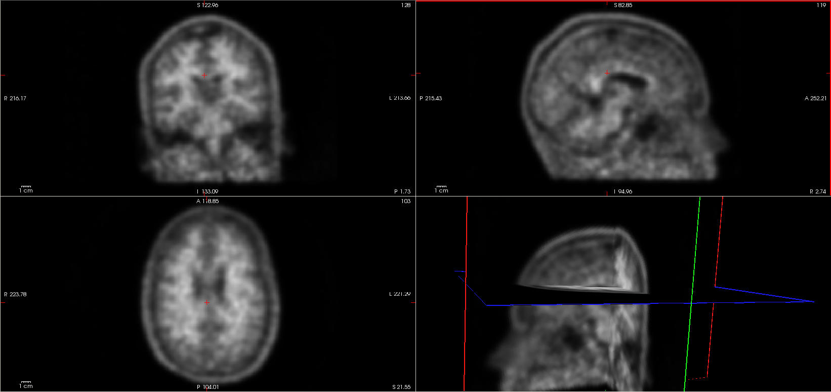
You can display the image with freeview ($ freeview sub-01_NAV_4D_pet.nii.gz &). Change the max value to around 500 (see the viewer options on the left). Play with the viewer and display options and explore your data. If you want to know more about freeview
How many frames are there ?
6 framesWhat can we say about the image ?
The low spatial resolution and low and Signal to Noise ratio (SNr) is due to physical constrains of the scanner. To overcome that, we can smooth the images and improve SNr and spatial resolution. Spatial noise is mostly Gaussian and roughly centered around zero. If that's true, then if we average across several voxels, the noise tends to go to zero, the signal tends to stay the same and the SNr is improved. For more information: http://imaging.mrc-cbu.cam.ac.uk/imaging/PrinciplesSmoothingClick to see answers
Smoothing and averaging the frames
In this step, we will do two things:
- smooth the image with a gaussian kernel (fwhm=6). As you saw, the image is highly pixelated (due to the characteristics of the acquisition). Thus images need to be smoothed prior analyses.
- compute the mean over time from the 4D image (i.e. mean of the
nframes to obtain a unique 3D volume for analyses/quantification of tracer uptake). Note that in some cases, you can have the entire dynamic scan from injection to the end of the scan. In that case you will take advantage of the different time frames and will not do this step.
Also, subjects could move during the acquisition of the frames. Data should be motion corrected. This could be perform several ways. One way is to compute the average volume of all the frames 5 minutes post-injection and then to register all the frames to his average. In this tutorial, frames are already realigned and you don’t have to perform this step.
$ fslmaths sub-01_NAV_4D_pet.nii.gz -kernel gauss 2.548 -fmean sub-01_NAV_4D_pet_smooth.nii.gz
$ fslmaths sub-01_NAV_4D_pet_smooth.nii.gz -Tmean sub-01_NAV_3D_pet_smooth.nii.gz
The first command can take several minutes.
It’s important to look at your data. The more the better. Display with freeview the files you just created sub-01_NAV_4D_pet_smooth.nii.gz and/or sub-01_NAV_3D_pet_smooth.nii.gz to check if these steps have been done properly.
PET registration to the anatomical image
This step transforms PET data from the PET-space to the freesurfer-space. PET data will thus be in the correct space to use anatomical data from freesurfer. This will allow to identify, for each subject, specific anatomical regions in the PET image. This anatomical information will be needed both for the scaling step (or quantitative normalization, see below) and analyses. The registration step, done with SPM, will create a new image (the coregistered one) with the prefix r.
$ mri_convert -i ../data/sub-01/sub-01_freesurfer/mri/T1.mgz -o sub-01_T1w.nii
$ gzip -d sub-01_NAV_3D_pet_smooth.nii.gz
$ cp ../scripts/sub-01/sub-01_coregister.m .
$ matlab -nodisplay < sub-01_coregister.m
$ gzip sub-01_NAV_3D_pet_smooth.nii
$ gzip sub-01_T1w.nii
$ gzip rsub-01_NAV_3D_pet_smooth.nii
$ fslmaths rsub-01_NAV_3D_pet_smooth.nii.gz -nan rsub-01_NAV_3D_pet_smooth.nii.gz
The matlab command can last several minutes.
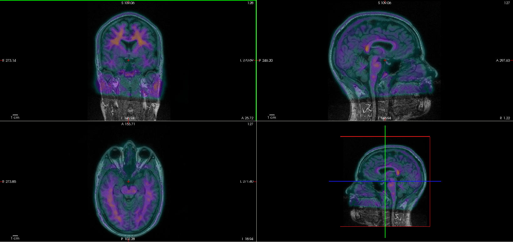
Check the quality of the registration. Open the T1w image and the registered PET image in the same viewer ($ freeview sub-01_T1w.nii.gz rsub-01_NAV_3D_pet_smooth.nii.gz &). Select the colormap “GE Color” for the registered PET image. Play with the opacity to check the registration quality.
Aparc_aseg atlas
Now that the PET image is in the freesurfer-space, it is possible to use freesurfer atlases.
$ mri_convert -i ../data/sub-01/sub-01_freesurfer/mri/aparc+aseg.mgz -o sub-01_atlas.nii.gz
$ freeview rsub-01_NAV_3D_pet_smooth.nii.gz sub-01_atlas.nii.gz:colormap=lut
Play with the opacity option. Information about the currently displayed data can be obtained by moving the mouse over the display window or by clicking to set the cursor. As the mouse is moved in the display window, the Cursor/Mouse sections on the bottom will display information about the voxel (or volume element) under the tip of the mouse arrow.
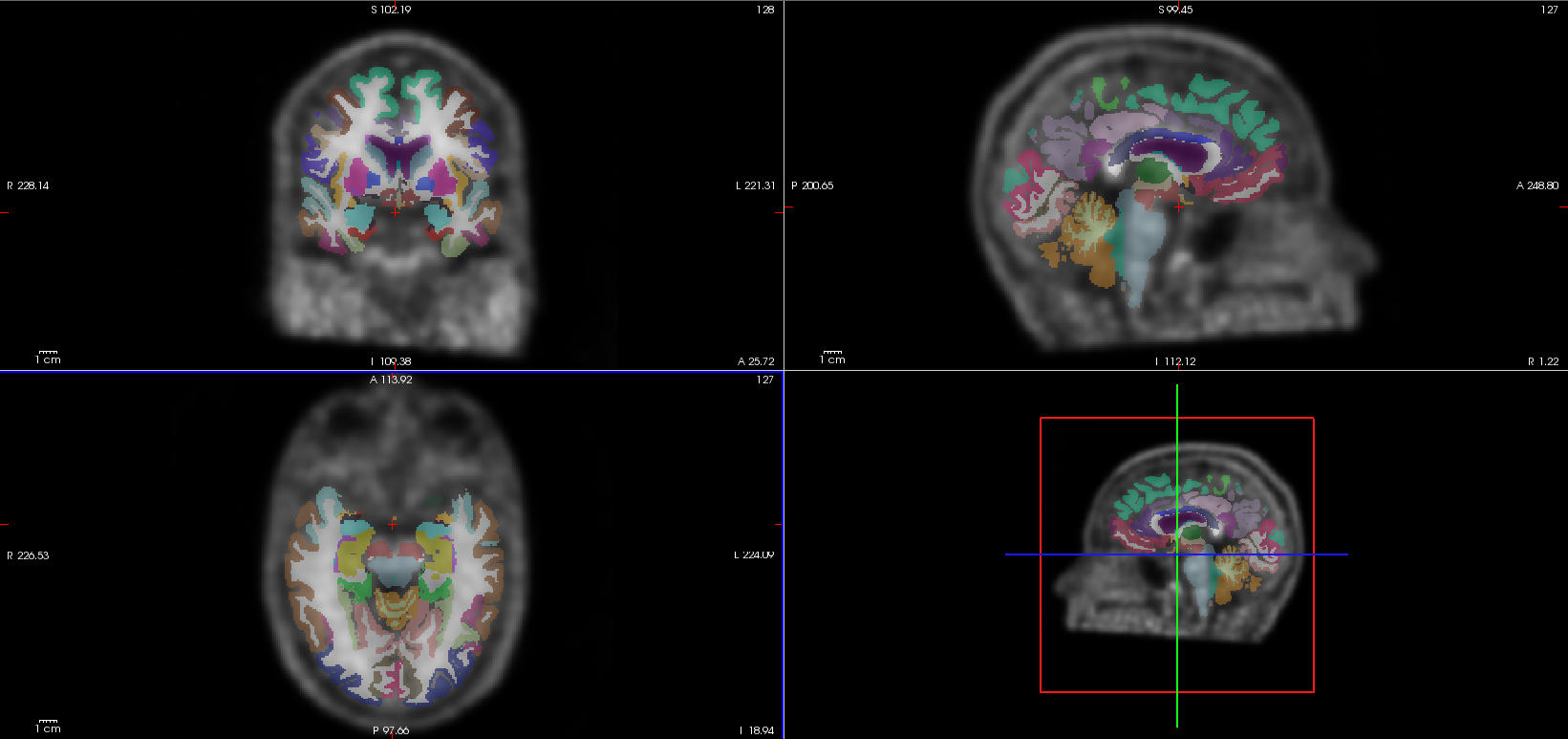
Which numbers correspond to the left and right cerebellum cortex ?
number 8 for the left cerebellum cortex and number 47 for the right cerebellum cortexStandardized Uptake Value ratio (SUVr)
Due to physiological differences, radioactivity concentration differs from one individual to another. Thus, to make the individuals comparable, a ratio is computed in which all the uptake values of the image are divided by the averaged uptake of a “reference region”. The reference region is chosen for being devoid of the targeted neuropathological alteration, in our example amyloid plaques. In other words, uptake value of the reference region should reflect only this physiological binding specific to each individual. This quantitative normalization (or scaling) step gives the “Standardized Uptake Value ratio” or SUVr.
In this example, we will use the cerebellum cortex as a reference region. We first need to create a mask of this region from the freesurfer atlas, then compute the average uptake inside this region and finally divide the PET image by this averaged value.
The reference region may change depending on the type of analysis, tracer or other reason. For example the whole cerebellum can be used to compute the average uptake.
Reference region creation and average computation
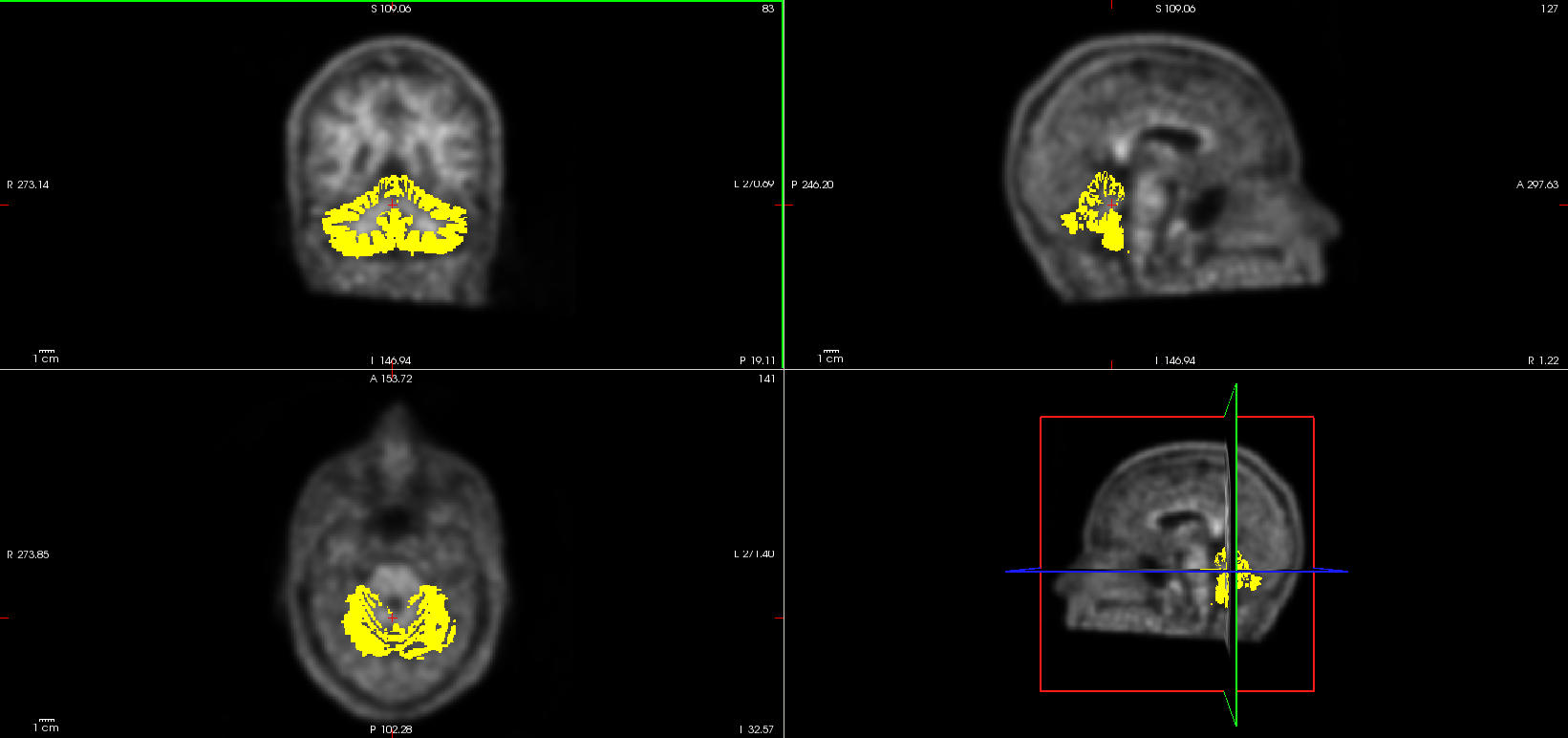
Note that, to isolate the left and right cerebellum cortex from the freesurfer aparc_aseg atlas, you need to identify their index (see above) as they need to be specified in the script (i.e. 8 for the left and 47 for the right cerebellum)
$ fslmaths sub-01_atlas.nii.gz -thr 8 -uthr 8 -bin sub-01_left-cerebellum-cortex.nii.gz
$ fslmaths sub-01_atlas.nii.gz -thr 47 -uthr 47 -bin sub-01_right-cerebellum-cortex.nii.gz
$ fslmaths sub-01_left-cerebellum-cortex.nii.gz -add sub-01_right-cerebellum-cortex.nii.gz -bin sub-01_cerebellum-cortex.nii.gz
$ fslmeants -i rsub-01_NAV_3D_pet_smooth.nii.gz -m sub-01_cerebellum-cortex.nii.gz -o sub-01_average_uptake_cerebellum-cortex.txt
Check the cerebellum cortex mask, open it on top of your registered PET image.
Scaling SUVr computation
PET image is divided (i.e. scaled) by the mean uptake of the reference region previously obtained.
$ cat sub-01_average_uptake_cerebellum-cortex.txt
$ fslmaths rsub-01_NAV_3D_pet_smooth.nii.gz -div <value> rsub-01_NAV_3D_pet_smooth_suvr.nii.gz
The first command print the average uptake of the cerebellum cortex. In the second command, you need to replace <value> by this average, it should be around 31.37 for this example with the NAV tracer. You now have the SUVr image.
Open the SUVr image on top of the T1w like in the PET registration step.
ROIs summary computation
You can now extract the SUVr from several regions. For this you need to refer to the freesurfer atlases.
$ mri_segstats --ctab-default --excludeid 0 --i rsub-01_NAV_3D_pet_smooth_suvr.nii.gz --seg sub-01_atlas.nii.gz --sum sub-01_summary_suvr.stats
The mri_segstats command can last several minutes. This freesurfer function computes several metrics (volume, mean, stddev, minimum, maximum and range) for each region of the atlas.
Here, we obtain the mean SUVr for each freesurfer aparc+aseg region. You can use other atlases or predefined masks to computed SUVr.